Ultimate Guide: Calculate Conveyor Belt Capacity (TPH)

How to calculate conveyor belt capacity in tons per hour

Getting capacity right is the difference between a conveyor that quietly does its job and one that spills, wears fast, and starves your plant. If you came here asking how to calculate conveyor belt capacity in tons per hour, the short answer is mass flow equals cross‑sectional area times belt speed times bulk density—then adjust for incline and geometry. The longer answer below shows the exact equations, the choices behind each variable, and a worked example you can replicate.

Key takeaways

Capacity is governed by Q = A × v × ρ. Use the correct bulk density (loose heap), not solid density.
For troughed belts, cross‑sectional area A depends on belt width, troughing angle, and material surcharge angle. Use recognized charts or a calculator.
On inclines, apply a cos α reduction; higher trough angles and favorable surcharge angles increase capacity.
Choose belt width for lump size first, then use speed for fine tuning—this improves containment, sealing, and cleaner life.
Verify in the field with timed load tests and document assumptions for density, speed, and geometry.

Core concepts and the TPH formula

In continuous conveying, mass flow is the product of how much material fits in the belt cross‑section and how quickly the belt moves that cross‑section past a point.

Mass flow (TPH) = 3600 × A × v × ρ_t
  
  Where: A = loaded cross‑section area (m²)
         v = belt speed (m/s)
         ρ_t = bulk density in tonnes per cubic metre (t/m³)
  
  Equivalent form using kg/m³:
  TPH = 3.6 × A × v × ρ_kg  (ρ_kg in kg/m³)

Engineering references present the same relationship; for example, the basic Q = ρ × A × v formulation is summarized by the Engineering ToolBox conveyor capacity page (accessed 2026), and a TPH‑ready framing with the 3.6 coefficient is discussed in West River Conveyors’ primer on TPH and belt widths (2024–2025 updates).

Troughed belt geometry: troughing and surcharge angles

On a three‑roll troughed belt, the material forms a heaped profile. Two angles matter:

Troughing angle: the side‑roll angle (commonly 30°–35°) that deepens the cross‑section.
Surcharge (dynamic) angle: the flowing surface angle on a moving belt, typically lower than the static angle of repose. For dry quarried stone and coal, ~15°–25% is common in practice.

Rather than derive A analytically every time, engineers reference width–speed charts created for a reference trough (often 35°) and a reference surcharge angle, then adjust when actual geometry differs. A clear explanation of this method—including incline corrections and capacity factors—is provided by MEKA Global’s belt conveyor capacity guide (2025).

Inclines and capacity factor

As the conveyor inclines by angle α, the effective cross‑section reduces. A standard correction is multiplying by cos α. Practical multipliers are modest at small angles (e.g., 10° ≈ 0.985; 20° ≈ 0.940). MEKA’s guide also describes a capacity factor (CF) to account for differences between your trough/surcharge combination and the reference charts.

Practical example: replicate the math step by step

Let’s run a representative case you can sanity‑check on paper and with a calculator.

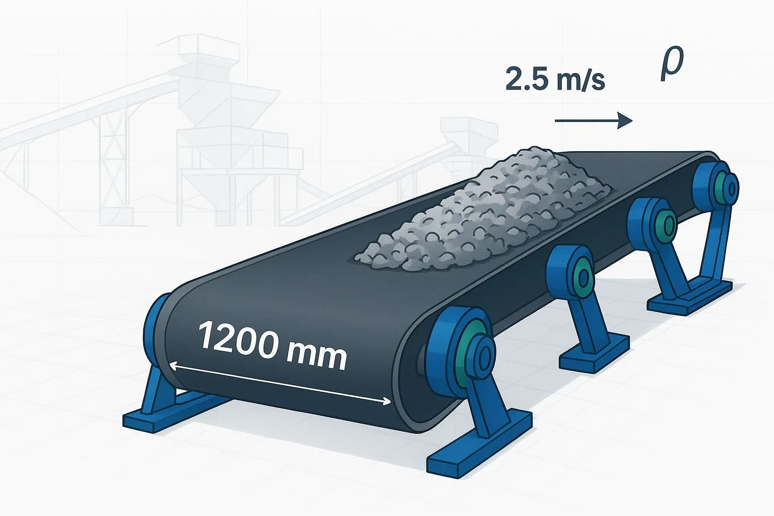
Belt width: 1200 mm
Troughing: 35° three‑roll (reference)
Belt speed v: 2.5 m/s
Bulk density ρ: 1.6 t/m³ (typical dense aggregate)
Incline α: 0° (horizontal)

Cross‑section area A: For a 1200 mm belt with a 35° trough and a typical surcharge, A is approximately 0.15 m² under reference conditions (public primers and charts converge on this order of magnitude; consult design charts for exact values).
Compute capacity in TPH using the tonne‑based form:

Volumetric flow = A × v = 0.15 × 2.5 = 0.375 m³/s
Mass flow in t/s = 0.375 × 1.6 = 0.600 t/s
TPH = 0.600 × 3600 = 2160 t/h

If the same conveyor ran at a 20° incline, apply cos 20° ≈ 0.940:

TPH_inclined ≈ 2160 × 0.940 ≈ 2030 t/h

You can repeat this workflow with your own parameters. For a chart‑based path (starting with volumetric capacity V in m³/h), compute TPH = V × ρ × cos α × CF as described in MEKA’s capacity method.

Tip: If you prefer a quick check with a pre‑set trough assumption, try the in‑browser Conveyor Belt Capacity Calculator. In project workflows, teams I’ve worked with often run the hand calc first, then validate with a tool.

Note on neutrality and components: In real RFQs and design reviews, teams often evaluate belts, idlers, and pulleys together with capacity. An experienced supplier like BisonConvey can be used as a reference point for component availability once you’ve pinned down width, speed, and duty—without changing the calculation principles above.

Selection and implementation guidelines

Before you commit to a width and speed, confirm physical and operational constraints. Think of capacity as a negotiation between “how much fits” and “how well it stays on the belt.”

Width vs. maximum lump size: Select belt width to accommodate the largest lumps first; a common heuristic keeps maximum lump at roughly one‑third to one‑half of belt width, depending on grading and loading. Public primers (e.g., MEKA) provide representative maxima by width.
Speed bands by material: For hard ore and sharp stone on 600–1200 mm belts, mid‑2 to mid‑3 m/s is common; wider belts in cleaner duties can run faster, but containment, wear, and cleaner ratings set limits. Practice notes on bands and trade‑offs appear in MEKA’s guide and in West River’s heavy construction engineering notes.
Trough angle and sealing: 30°–35° troughs balance capacity and containment in many plants. Deeper troughs raise capacity but demand careful transition design and skirt sealing.

Below is an indicative lookup for a single operating point (horizontal, 35° trough, v = 2.5 m/s, ρ = 1.6 t/m³). It scales the 1200 mm example proportionally for illustration only. Exact design must use proper cross‑section charts or a calculator.

Use this table strictly for order‑of‑magnitude checks; real A does not scale exactly with width squared because edge clearances and trough geometry complicate the shape. For authoritative methods, see MEKA’s explanation and the basic Q = ρAv foundation in Engineering ToolBox.

Problems and troubleshooting

Even good math can underperform in the field if assumptions drift or containment is weak. Watch for these recurring issues:

Using solid density instead of bulk heap density (overstates capacity). Public density references such as Engineering ToolBox list bulk ranges for coal and aggregates.
Over‑speeding to chase TPH, which increases dust, spillage sensitivity, idler RPM/wear, and can exceed cleaner ratings. West River’s primers discuss speed versus containment.
Ignoring lump‑size limits for the chosen width, causing point loading, impact damage, or persistent spillage.
Forgetting incline reductions; even 20° cuts effective capacity by about 6%.

Commissioning checklist for capacity verification

Confirm belt speed under load (tachometer or encoder trend), not just nameplate.
Measure bulk heap density with a field sample and bucket method; update ρ in your calc.
Time a weighed throughput test (truck scale or belt scale cross‑check) over a stable period.
Inspect loading zone: free edge clearance, skirtboard height/pressure, and transition geometry.
Check idler spacing and rotation in the load zone; adjust if sag or vibration changes A.
Document assumptions, test conditions, and corrections (incline, CF) in the handover pack.

For sealing details and containment heuristics, Martin Engineering’s practitioner posts (e.g., idler classes and skirting practices) provide accessible, standards‑aware guidance; see the discussion in Martin Engineering’s CEMA explainer (2023) and extend your plant practices accordingly.

Best practices that hold up in plants

Design width for lumps and containment first, then tune speed. This often reduces dust and improves cleaner life.
Match idler duty class to load and environment; sealed-for-life bearings help only if ingress is controlled.
Validate A with either a reputable chart method and CF adjustment or a calculator; do not extrapolate far from reference geometry.
Keep incline corrections explicit in your calcs and drawings.
Train and document: include your density source, test method, and the final TPH check in commissioning records.

For deeper dives on capacity versus containment trade‑offs in sand and gravel systems, this guide provides context and visual cues: Custom Conveyor Systems for Sand & Gravel — Ultimate Guide.

Why the standards matter (without reproducing protected tables)

Industry practice aligns around methods outlined in CEMA (Belt Conveyors for Bulk Materials, 7th ed.) and referenced internationally alongside ISO conventions (e.g., pulley diameters and power verification). While detailed tables are proprietary, the workflow here—Q = A × v × ρ, trough reference charts, incline correction, and verification—follows that body of practice as echoed by the public primers cited above.

Wrapping up: How to calculate conveyor belt capacity in tons per hour

Here’s the practical summary:

Start with Q = A × v × ρ (TPH = 3600 × A × v × ρ_t, or 3.6 × A × v × ρ_kg). Use bulk heap density.
Determine A from a recognized 35° trough reference (or your actual geometry) and correct for incline and capacity factors.
Choose width for lumps and containment; apply speed within the material‑appropriate band; verify in the field.

If you want a quick, standards‑aware check, run your numbers through the Conveyor Belt Capacity Calculator and compare against your hand calc. When it’s time to select belts, idlers, and pulleys for your duty, you can open an engineer‑to‑engineer conversation with BisonConvey for custom, application‑specific options.